How to Read a Mosaic Plot: The Hidden Art of Visualizing Complex Data
Mosaic plots are often overlooked in the toolkit of data analysts, yet they offer a uniquely intuitive way to dissect complex relationships between categorical variables. Unlike bar charts or pie charts, which simplify data into single dimensions, a mosaic plot layers multiple variables into a single, spatially proportional diagram. This allows viewers to instantly grasp conditional probabilities, dependencies, and even subtle asymmetries in datasets. The ability to read mosaic plot structures with precision can transform how researchers, marketers, and policymakers interpret survey responses, experimental outcomes, or demographic distributions.
What makes mosaic plots particularly compelling is their capacity to reveal interactions that scatterplots or heatmaps might obscure. For instance, a well-constructed mosaic plot can show not just that "Group A performs better than Group B," but why—by visualizing how subgroups within A and B behave differently across multiple conditions. This level of granularity is why statisticians and data scientists increasingly turn to mosaic plots when dealing with contingency tables or stratified data. However, mastering their interpretation requires understanding the underlying geometry and the rules governing their construction.
The challenge lies in translating the plot’s spatial proportions into actionable insights. A mosaic plot’s rectangles are sized proportionally to their frequencies, but their arrangement—whether stacked horizontally, vertically, or nested—encodes deeper relationships. Misreading these proportions can lead to incorrect conclusions, such as overestimating the strength of an association or ignoring confounding variables. To read mosaic plot effectively, one must decode these visual cues: the width of a rectangle reflects its marginal frequency, while its height or depth indicates conditional probabilities. This guide demystifies the process, from historical roots to modern applications, ensuring you can extract maximum value from these underrated visualizations.
The Complete Overview of Mosaic Plots
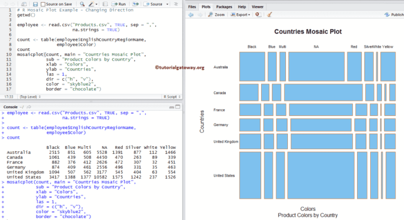
Mosaic plots are a class of statistical graphics designed to represent the structure of categorical data in a way that preserves both marginal and conditional distributions. Developed as an extension of the mosaic display concept by Hartigan and Kleiner in the 1980s, they extend beyond simple bar charts by incorporating multiple dimensions into a single, cohesive layout. The core innovation lies in their ability to handle contingency tables—where rows and columns represent categorical variables—by partitioning space proportionally to observed frequencies. This makes them particularly useful for datasets where relationships between variables are not immediately obvious, such as survey responses, market segmentation, or experimental outcomes.The visual appeal of mosaic plots stems from their adherence to the principles of proportional ink, where the area of each rectangle corresponds to the frequency of a specific combination of categories. Unlike treemaps, which prioritize hierarchical nesting, mosaic plots emphasize association by aligning rectangles along axes that represent the variables being compared. For example, a plot analyzing voter demographics might show how age groups (rows) distribute across political affiliations (columns), with the size of each rectangle revealing the strength of each combination. This spatial encoding allows analysts to read mosaic plot structures at a glance, identifying outliers, clusters, or unexpected interactions without relying on numerical tables.
Historical Background and Evolution
The origins of mosaic plots trace back to the early 20th century, when statisticians sought ways to visualize complex contingency tables more intuitively. Pioneers like William S. Gosset ("Student") and Ronald Fisher laid the groundwork for graphical methods to represent categorical data, but it wasn’t until the 1980s that mosaic plots emerged as a distinct tool. Hartigan and Kleiner’s 1981 paper introduced the concept as a means to "see" the structure of a table by partitioning space into rectangles whose areas reflect joint frequencies. Their work built on earlier ideas from marimekko charts (used in business for stacked bar visualizations) but added the critical innovation of proportional scaling.The evolution of mosaic plots accelerated with advancements in computational graphics. By the 1990s, software like R (via the `vcd` package) and Python (`statsmodels`) made it feasible to generate dynamic, interactive versions of these plots. This democratized their use, allowing researchers to read mosaic plot outputs without relying on static, hand-drawn diagrams. Modern applications extend beyond academia: marketers use them to segment customer bases, epidemiologists analyze disease prevalence across demographics, and social scientists study behavioral patterns. The adaptability of mosaic plots—whether in static reports or dashboards—has cemented their role as a bridge between raw data and actionable insights.
Core Mechanisms: How It Works
At their core, mosaic plots operate on two fundamental principles: proportional area and variable alignment. The area of each rectangle in the plot is directly proportional to the frequency of the corresponding category combination in the contingency table. For instance, if "Young Males" represent 20% of a dataset, their rectangle will occupy 20% of the total plot area. This ensures that visual comparisons are both accurate and immediately perceptible. The alignment of rectangles along axes corresponding to the variables being analyzed (e.g., rows for one category, columns for another) allows viewers to read mosaic plot structures by tracing relationships across dimensions.Table of Contents
- The Complete Overview of Mosaic Plots
- Historical Background and Evolution
- Core Mechanisms: How It Works
- Key Benefits and Crucial Impact
- Major Advantages
- Comparative Analysis
- Future Trends and Innovations
- Conclusion
- Comprehensive FAQs
- Q: What software tools can I use to create mosaic plots?
- Q: How do I know if a mosaic plot is correctly constructed?
- Q: Can mosaic plots handle more than two categorical variables?
- Q: What’s the difference between a mosaic plot and a stacked bar chart?
- Q: How can I improve the readability of a complex mosaic plot?
- Q: Are mosaic plots suitable for time-series data?
The construction process begins with a contingency table, where rows and columns define the categorical variables. The plot then partitions space such that:
1. Marginal frequencies are represented by the total width or height of rectangles in each row/column.
2. Conditional frequencies are shown by the relative sizes of sub-rectangles within a row or column.
3. Associations between variables are visualized through deviations from expected uniformity (e.g., a wider-than-expected rectangle suggests a stronger relationship).
For example, in a plot analyzing "Education Level vs. Income Bracket," a disproportionately large rectangle for "College Graduates in High Income" would indicate a positive association, while a smaller-than-expected rectangle for "High School Dropouts in Low Income" might reveal an unexpected pattern. This spatial logic is what enables analysts to interpret mosaic plot data without delving into raw numbers.
Key Benefits and Crucial Impact
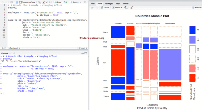
Mosaic plots excel where traditional tables and charts fall short: they simultaneously display marginal distributions, conditional probabilities, and interactions between variables. This multifaceted approach is particularly valuable in fields like medicine, where understanding how multiple risk factors (e.g., age, gender, lifestyle) interact to influence outcomes can save lives. Unlike heatmaps, which rely on color gradients that can distort perception, mosaic plots use area and position to convey information objectively. Their ability to handle high-dimensional data—without the clutter of overlapping lines or ambiguous color scales—makes them indispensable for exploratory data analysis.The impact of mosaic plots extends to decision-making. In market research, for example, a mosaic plot might reveal that a product’s adoption varies not just by age but by age combined with income and region—insights that a simple bar chart would miss. Similarly, in public policy, they can highlight disparities in service access across demographic groups, guiding resource allocation. The clarity of mosaic plots lies in their adherence to the preattentive attributes of human perception: we intuitively grasp area and position better than abstract numbers or arbitrary color mappings. This makes them a powerful tool for communicating complex findings to stakeholders who may lack statistical expertise.
"A mosaic plot is not just a picture of data; it is a conversation between the analyst and the data itself. The way rectangles align and diverge tells a story that numbers alone cannot." — John Hartigan, Statistician & Visualization Pioneer
Major Advantages
- Multidimensional Clarity: Mosaic plots can represent interactions between three or more categorical variables in a single visualization, whereas scatterplots or heatmaps struggle with dimensionality.
- Proportional Accuracy: The area of each rectangle directly reflects its frequency, eliminating the risk of misinterpretation from skewed axes or arbitrary scaling.
- Conditional Insights: By aligning rectangles along variable axes, analysts can read mosaic plot structures to identify conditional dependencies (e.g., "Does the effect of Variable A depend on the level of Variable B?").
- Outlier Detection: Rectangles that deviate significantly from expected proportions (based on marginal frequencies) signal potential outliers or unexpected patterns.
- Scalability: Mosaic plots adapt to datasets of varying sizes, from small survey responses to large-scale demographic studies, without losing interpretability.
Comparative Analysis
While mosaic plots offer unique advantages, other visualization tools serve distinct purposes. Below is a comparison of mosaic plots with alternative methods for categorical data:| Feature | Mosaic Plot | Heatmap |
|---|---|---|
| Primary Use Case | Exploring associations and conditional distributions in contingency tables. | Displaying intensity or correlation values across a grid (often for continuous or binned data). |
| Strengths | Accurate proportional representation; clear marginal/conditional relationships. | Good for highlighting extreme values or gradients; works well with large datasets. |
| Weaknesses | Can become cluttered with many categories; less intuitive for non-technical audiences. | Color scaling can distort perception; less effective for showing exact frequencies. |
| Best For | Analyzing survey data, market segmentation, or experimental outcomes with clear categorical variables. | Correlation matrices, gene expression data, or spatial heatmaps. |
Future Trends and Innovations
The future of mosaic plots lies in their integration with interactive and dynamic visualization tools. As data volumes grow, static mosaic plots risk becoming unwieldy, but advancements in web-based platforms (e.g., Plotly, D3.js) are enabling interactive mosaic plot explorations. Users can now hover over rectangles to see exact frequencies, filter variables dynamically, or animate transitions between datasets. This interactivity not only enhances the ability to read mosaic plot structures but also makes them accessible to broader audiences.Another promising trend is the fusion of mosaic plots with machine learning. Algorithms could automatically highlight anomalous rectangles or suggest optimal variable groupings, reducing the manual effort required to interpret complex datasets. Additionally, the rise of augmented reality (AR) could allow analysts to "step into" a mosaic plot, examining 3D representations of categorical relationships in immersive environments. As these innovations unfold, mosaic plots may transition from niche statistical tools to mainstream data storytelling platforms, bridging the gap between raw data and strategic decision-making.

Conclusion
Mosaic plots remain one of the most underutilized yet powerful tools in data visualization, offering a level of detail and clarity that few alternatives can match. Their ability to read mosaic plot structures—revealing hidden patterns in categorical data—makes them indispensable for researchers, analysts, and decision-makers. The key to leveraging their full potential lies in understanding their geometric principles and applying them to real-world datasets. Whether analyzing market trends, healthcare outcomes, or social behaviors, mosaic plots provide a visual language that transcends numerical tables and simplistic charts.As data continues to grow in complexity, the demand for intuitive, scalable visualization techniques will only increase. Mosaic plots are well-positioned to meet this need, especially as they evolve with interactive technologies and machine learning. By mastering the art of interpreting mosaic plot visualizations, professionals can unlock deeper insights, communicate findings more effectively, and drive decisions with confidence.
Comprehensive FAQs
Q: What software tools can I use to create mosaic plots?
A: Popular tools include R (via the `vcd` and `mosaic` packages), Python (`statsmodels`, `pandas` with `plotnine`), and specialized visualization platforms like Tableau or Plotly. For quick analysis, online tools like DataDesk also support mosaic plot generation.
Q: How do I know if a mosaic plot is correctly constructed?
A: A properly constructed mosaic plot will have rectangles whose areas sum to 100% of the total frequency, and the marginal proportions (row/column totals) should match the observed data. Use software validation checks or compare the plot’s area proportions to the raw contingency table.
Q: Can mosaic plots handle more than two categorical variables?
A: Yes, but the complexity increases. Three-dimensional mosaic plots (using depth) or layered plots can represent three variables, though interpretability may decline. For higher dimensions, consider treemaps or parallel coordinates as alternatives.
Q: What’s the difference between a mosaic plot and a stacked bar chart?
A: Mosaic plots use proportional area to represent frequencies, while stacked bars rely on height. Mosaic plots also align rectangles along variable axes, making conditional relationships clearer. Stacked bars are better for comparing totals across categories, whereas mosaic plots excel at showing interactions.
Q: How can I improve the readability of a complex mosaic plot?
A: Simplify by reducing the number of categories, use color sparingly (only for grouping, not encoding data), and add annotations for key rectangles. Interactive tools can help users explore subsets of the data dynamically.
Q: Are mosaic plots suitable for time-series data?
A: Not directly. Mosaic plots are designed for categorical cross-sections, not temporal trends. For time-series, consider line charts, area plots, or small multiples of mosaic plots over time periods.
Leave a Comment
Comments are moderated before appearing. The data you submit is processed according to the Privacy Policy of Filmfestivalcircuit.